File:Tautochrone curve.gif

Summary

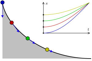
A tautochrone curve is the curve for which the time taken by an object sliding without friction in uniform gravity to its lowest point is independent of its starting point. Here, four points at different positions reach the bottom at the same time.

In the graphic, s represents arc length, t represents time, and the blue arrows represent acceleration along the trajectory. As the points reach the horizontal, the velocity becomes constant, the arc length being linear to time. Date 9 May 2007; new version August 2009 Source Own work Author Claudio Rocchini

rewritten by Geek3 GIF development

This plot was created with Matplotlib.

Source code Python code

1. !/usr/bin/python
2. -*- coding: utf8 -*-

animation of balls on a tautochrone curve

import os import numpy as np import matplotlib.pyplot as plt import matplotlib.patches as patches from matplotlib import animation from math import *

1. settings

fname = 'Tautochrone curve' width, height = 300, 200 nframes = 80 fps=25

balls = [ {'a':1.0, 'color':'#0000c0'}, {'a':0.8, 'color':'#c00000'}, {'a':0.6, 'color':'#00c000'}, {'a':0.4, 'color':'#c0c000'}]

def curve(phi):

   x = phi + sin(phi)
   y = 1.0 - cos(phi)
   return np.array([x, y])

def animate(nframe, empty=False):

   t = nframe / float(nframes - 1.)
   
   # prepare a clean and image-filling canvas for each frame
   fig = plt.gcf()
   fig.clf()
   ax_canvas = plt.gca()
   ax_canvas.set_position((0, 0, 1, 1))
   ax_canvas.set_xlim(0, width)
   ax_canvas.set_ylim(0, height)
   ax_canvas.axis('off')
   
   # draw the ramp
   x0, y0 = 293, 8
   h = 182
   npoints = 200
   points = []
   for i in range(npoints):
       phi = i / (npoints - 1.0) * pi - pi
       x, y = h/2. * curve(phi) + np.array([x0, y0])
       points.append([x, y])
   
   rampline = patches.Polygon(points, closed=False, facecolor='none',
                      edgecolor='black', linewidth=1.5, capstyle='butt')
   points += [[x0-h*pi/2, y0], [x0-h*pi/2, y0+h]]
   
   ramp = patches.Polygon(points, closed=True, facecolor='#c0c0c0', edgecolor='none')
   
   # plot axes
   plotw = 0.5
   ax_plot = fig.add_axes((0.47, 0.46, plotw, plotw*2/pi*width/height))
   ax_plot.set_xlim(0, 1)
   ax_plot.set_ylim(0, 1)
   for b in balls:
       time_array = np.linspace(0, 1, 201)
       phi_pendulum_array = (1 - b['a'] * np.cos(time_array*pi/2))
       ax_plot.plot(time_array, phi_pendulum_array, '-', color=b['color'], lw=.8)
   ax_plot.set_xticks([])
   ax_plot.set_yticks([])
   ax_plot.set_xlabel('t')
   ax_plot.set_ylabel('s')
   
   ax_canvas.add_patch(ramp)
   ax_canvas.add_patch(rampline)
   
   for b in balls:
       # draw the balls
       phi_pendulum = b['a'] * -cos(t * pi/2)
       phi_wheel = 2 * asin(phi_pendulum)
       phi_wheel = -abs(phi_wheel)
       x, y = h/2. * curve(phi_wheel) + np.array([x0, y0])
       ax_canvas.add_patch(patches.Circle((x, y), radius=6., zorder=3,
                           facecolor=b['color'], edgecolor='black'))
       ax_plot.plot([t], [1 + phi_pendulum], '.', ms=6., mec='none', mfc='black')
       
       v = h/2. * np.array([1 + cos(phi_wheel), sin(phi_wheel)])
       vnorm = v / hypot(v[0], v[1])
       # in the harmonic motion, acceleration is proportional to -position
       acc_along_line = 38. * -phi_pendulum * vnorm
       ax_canvas.arrow(x, y, acc_along_line[0], acc_along_line[1],
                head_width=6, head_length=6, fc='#1b00ff', ec='#1b00ff')

fig = plt.figure(figsize=(width/100., height/100.)) print 'saving', fname + '.gif'

1. anim = animation.FuncAnimation(fig, animate, frames=nframes)
2. anim.save(fname + '.gif', writer='imagemagick', fps=fps)

frames = [] for nframe in range(nframes):

   frame = fname + '_{:02}.png'.format(nframe)
   animation.FuncAnimation(fig, lambda n: animate(nframe), frames=1).save(
       frame, writer='imagemagick')
   frames.append(frame)

1. assemble animation using imagemagick, this avoids dithering and huge filesize

os.system('convert -delay {} +dither +remap -layers Optimize {} "{}"'.format(

   100//fps, ' '.join(['"' + f + '"' for f in frames]), fname + '.gif'))

for frame in frames:

   if os.path.exists(frame):
       os.remove(frame)

Licensing

This work is licensed under the Creative Commons Attribution-ShareAlike 2.5 License. https://creativecommons.org/licenses/by-sa/2.5/CC-BY-SA-2.5Creative Commons Attribution-ShareAlike 2.5truetrue